ABSTRACT
The paper will first give a brief description of the economy of Malaysia. This will be followed by a discussion of our econometric model. This would include testing the reliability of our model, which may warrant the use of several different tests. We shall also examine the significance of our beta coefficients to determine whether or not they have an impact on fertility rates. Lastly, this article shall also examine the available literature on this topic to verify whether our results or consistent with the finding of others.
INTRODUCTION:
Malaysia’s economy transitioned from being heavily dependent upon the export of raw materials such as tin and rubber to being one of the most diversified, robust and fastest-growing economies in South East Asia. Regardless of the structural changes that Malaysia underwent, much of its net exports are accounted for by the export of raw materials such as rubber, palm oil, natural gas, and petroleum. Malaysia is considered an attractive opportunity by Japanese and Taiwanese investors due to its comparative advantage of the cheap yet educated labour force, well-built infrastructure, and political stability (Bee 2021).
According to an article by Jati Kasuma, Malaysia had attained economic growth averaging about 5.8 per cent during a period of sustained economic growth that had continued for the past three decades. This growth had been attributed to structural economic changes, which “transformed Malaysia into a developing country with a multisector economy backed by strong performances of the manufacturing and services sector” (Kasuma). In the same study, the link between Malaysia’s economic performance and the performance of the global economy was also examined. They concluded that even though Malaysia did boast a relatively strong and stable economic growth, it was still reliant upon global conditions making it prone to external risks and shocks. When observing data about economic growth from 1976 to 2016, we find evidence of this statement. For example, there was a decline in economic growth from 2007-2009, which could be attributed to the global recession caused by the housing market bubble in the USA.
DATA AND METHODOLOGY:
In econometric models, we are usually concerned with an effect that one independent variable might have on another variable, called a dependent variable. However, the data we have might not allow us to make inferential claims as even though there might be a correlation. However, these correlations might have been caused by another variable, called a lurking variable, which affects both the dependent and the independent variable.
To counter this problem, we can make use of control variables. For example, we are interested in knowing whether female labour force participation (PART) affects fertility rates (FERT), but we suspect that GDP per capita (GDPC) is a lurking variable. Therefore, we would include GDP per capita into our model by introducing another independent variable. This will help us isolate the effects of GDPC and PART on FERT and will allow us to make inferential claims.
The country chosen for our analysis is Malaysia, which is located in South East Asia. One factor which led to our choice was that the data was readily available and consistent. Other Asian countries, such as Bangladesh and Pakistan, lack data for many years. Secondly, Malaysia enjoys a lot of ethnic diversity, which can help us generalize the findings of this study to other regions such as China and India. The population composition of Malaysia shows that international immigrants, especially those from China and India, came to constitute about thirty-six per cent and eleven per cent, respectively while only fifty-three per cent could be classified as Malay(Bee).
Analysis:

FERT is the total fertility rate. We will treat this as our dependent variable.
B0 is the slope parameter for the population.
B1 will tell us the change in fertility rates, which can be attributed to a change in the percentage of the total population living in urban areas (URBAN)
B2 represents the change in FERT due to a change in female labour force participation rate (PART)
B3 is the change in FERT due to the change in gross domestic product per capita (GDPC)
U will serve as our error term for this model. It contains all the unobserved variables which might impact fertility rates.
When we run our regression of the aforementioned model, we get the following results:
| (1) | |
| VARIABLES | FERT |
| URBAN | -0.0957*** |
| (0.00806) | |
| PART | 0.0120 |
| (0.0101) | |
| GDPC | 0.000110*** |
| (3.71e-05) | |
| Constant | 7.358*** |
| (0.630) | |
| Observations | 29 |
| R-squared | 0.988 |
However, one may notice the absurdity in our model by looking at its R-squared, which stands at around 98.8%. This, in theory, would mean that our model explains close to 99 per cent of the variation in our data, which is really not possible.
One possible explanation for the inflated R-square is the correlation with time. This problem exists in time series data when the previous trends of a particular variable influence the future behaviour of the variable. Hence to deal with this issue, we have to detrend our data to remove the correlation between a variable and time. We do this by regressing time on each variable in our model individually. As there are four variables, we will have to run a total of four regressions. For example, we may regress time(t) on FERT and calculate its residuals; then we will regress t on URBAN and again calculate the residuals and so on.
Now we have four new variables, namely, FERTr , URBANr, PARTr, and GDPCr. The r, in the end, will be used to indicate residuals for that variable. For instance, FERTr would then mean residuals from the regression of t on FERT. Additionally, it might also be a good idea to include a lagged variable of FERTr to control for any variations in fertility rates caused by previous trends. Omitting such a variable might lead to omitted variable bias.
We now have a new model:

When we run the regression, we get the following results:
| (1) | |
| VARIABLES | FERTr |
| URBANr | -0.0359*** |
| (0.00798) | |
| PARTr | -0.0164*** |
| (0.00538) | |
| GDPCr | 5.22e-05*** |
| (1.75e-05) | |
| lag_FERTr | 0.965*** |
| (0.0781) | |
| Constant | 0.0301*** |
| (0.00576) | |
| Observations | 29 |
| Adjusted R-squared | 0.982 |
Standard errors in parentheses
*** p<0.01, ** p<0.05, * p<0.1
Individual significance test:
To test whether each of the coefficients is statistically significant, we must observe their P-values. Our hypothesis will be:
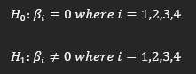
Using the P-value approach, we find that all our dependent variables are statistically significant at the 5% level.
Joint significance test:
Unfortunately, the usual T-stat approach does not work in the case of multiple restrictions. Therefore, we use the F-statistic instead. The method makes use of 2 models, unrestricted and restricted. The former contains the original model, whereas the latter removes the variables we may suspect hold no significance to our model. Our hypothesis in such a test is as follows:
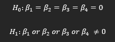
When we run the F-test, we obtain a nearly zero P-value, which informs us that our model is overall significant.
Breusch Pagan test:
The Breusch Pagan test (1979) helps us detect the presence of heteroskedasticity in our regression. If our assumption of constant variance amongst the error term is violated, it could affect the efficiency of our model and lead to a bias in our standard errors, and a wrong conclusion might ensue.


When we run the test, we get a chi-square statistic of 4.34 with a P-value of 0.95, and hence we fail to reject the null. This implies there is no heteroskedasticity present in our model. If it was present, then to counter this issue, we can make use of robust standard errors instead to check if our results vary from those of our previous model.
| (1) | |
| VARIABLES | FERTr |
| URBANr | -0.0359*** |
| (0.00836) | |
| PARTr | -0.0164** |
| (0.00619) | |
| GDPCr | 5.22e-05*** |
| (1.32e-05) | |
| lag_FERTr | 0.965*** |
| (0.0543) | |
| Constant | 0.0301*** |
| (0.00472) | |
| Observations | 29 |
| R-squared | 0.985 |
Robust standard errors in parentheses
*** p<0.01, ** p<0.05, * p<0.1
It is important to note that although the P-values have changed, our interpretation based on the previous model remains valid as the significance of the variables is still the same.
Durbin-Watson test:
The Durbin-Watson test allows us to test our residuals for serial correlation at lag one. This can help us identify whether previous trends of a variable influence its future value. For this test, our hypothesis will be as follows:


When we run the test, we obtain a d-stat of 0.919, which implies that there is a positive serial correlation.
When we add an additional explanatory variable, such as GOVEXPr, which represents government expenditure, we obtain the following results:
| (1) | (2) | |
| VARIABLES | FERTr | FERTr |
| URBANr | -0.0359*** | -0.0289*** |
| (0.00798) | (0.00617) | |
| PARTr | -0.0164*** | -0.0161*** |
| (0.00538) | (0.00403) | |
| GDPCr | 5.22e-05*** | 4.76e-05*** |
| (1.75e-05) | (1.32e-05) | |
| GOVEXPr | 0.0160*** | |
| (0.00360) | ||
| lag_FERTr | 0.965*** | 0.985*** |
| (0.0781) | (0.0586) | |
| Constant | 0.0301*** | 0.0579*** |
| (0.00576) | (0.00758) | |
| Observations | 29 | 29 |
| Adjusted R-squared | 0.982 | 0.990 |
Standard errors in parentheses
*** p<0.01, ** p<0.05, * p<0.1
The above model tells us that the beta coefficient of government expenditure is statistically significant. Moreover, instead of using the usual R-squared, in the above chart, we have included adjusted R-squared instead. As adjusted R-square penalizes for adding on irrelevant variables, we can conclude that it is, in fact, worth adding GOVEXPr as it increases our adjusted R-squared.
LITERATURE REVIEW AND CONCLUSION:
Throughout the course of this paper, we have examined the impact of different variables like ‘percentage of the total population living in urban areas,’ ‘female labour force participation rate,’ general government expenditure as a percentage of GDP’, and ‘GDP per capita’ on fertility rates in a developing country like Malaysia.
Urban population (% of total)
A study done by Audrey Siah and Grace Lee regarding the link between female labour force participation, infant mortality, and fertility rates in Malaysia might help us explicate the impact on the fertility rate that a country’s regional structure might have (Siah and Lee, 2015). According to one hypothesis, where child mortality rates are high, fertility rates are higher to ensure at least some of the children survive. As people migrate to urban areas that consist of better healthcare, child mortality rate decreases, and hence fertility rate decreases in tandem. Rosenzweig and Schultz (1985), for example, have also analyzed the link between fertility rates and infant mortality (Rosenzweig and Schultz, 1985). Moreover, it is also possible to apply Ghatak’s (1995) findings to our study, which states that fertility rates are higher in developing countries due to a lack of social services for the elderly, in which case children are treated as investments (Ghatak, 1995). Due to urbanization, family sizes shrink as children move out when they get married. Hence children are no longer seen as an investment, which might cause the negative relationship between URBAN and FERT. As we have seen, the coefficient of URBAN is negative, which is on par with our theory. As the percentage of the total population living in urban areas increase by one percentage point, the fertility rate decreases by 0.0438 percentage points on average.
Female labour force participation
The same study by Siah and Lee might also explain the link between female labour participation and fertility rates. Although the link has been examined by many scholars, however, the conclusion remains indecisive. The relationship between fertility and female employment is ambiguous, as it is still debated whether the link is positive or negative. Advocates for the former such as Rindfuss et al. (2000), use the ‘role incompatibility hypothesis’ to explain how the role of a woman as a mother hinders her role as an employee (Rindfuss, 2000). In this theory, the two jobs, i.e., childbearing and formal employment, negatively affect each other. On the other hand, scholars like Bernhardt (1993) have argued in favour of a positive link between the two variables by deploying the ‘societal response hypothesis’, which states that mothers who are part of the labour force are better able to provide for their children, hence in this regard fertility and female employment reinforce each other (Bernhardt, 1993). The results of our research seem to reinforce the ‘societal response hypothesis.’ As female participation rate increases by one percentage point, fertility rates decrease by 0.0175 percentage points on average.
GDP per capita
According to Weil (2013), when an economy gets more prosperous, it is faced with two opposing forces that can either cause a negative or a positive impact on fertility (Weil, 2013) . The income effect assumes children to be a normal good. In this regard, when a family’s income increases, they prefer more of the normal good, i.e. more children. On the other hand, the substitutional effect takes into account the opportunity cost of raising children, which can be stated in terms of income lost due to diverting energy and resources away from the labour force to raising kids instead. Hence in countries where the Income effect is greater than the substitutional effect, an increase in per capita income might lead to an increase in fertility rates. Such is the case with Malaysia, as we observe a positive relationship between GDPC and FERT.
Government expenditure
As previously mentioned, economic development may be affiliated with higher fertility rates, especially in countries where the income effect is greater than the substitution effect. An increase in government expenditure may cause an increase in healthcare facilities, which might lead to an increase in fertility rates.
Reference List
Bee, O., 2021. Malaysia | Facts, Geography, History, & Points Of Interest. [online] Encyclopedia Britannica. Available at: <https://www.britannica.com/place/Malaysia> [Accessed 11 January 2021].
Bernhardt, E.M. 1993. “Fertility and employment.” European Sociological Review 9 (1), 25– 42.
Breusch, T. S., and A. R. Pagan. “A Simple Test for Heteroscedasticity and Random Coefficient Variation.” Econometrica, vol. 47, no. 5, 1979, pp. 1287–1294. JSTOR, www.jstor.org/stable/1911963. Accessed 11 Jan. 2021.
Ghatak, S. 1995. “Fertility in the Pacific island countries. Introduction to Development Economics.” Routledge, London.
Kasuma, Jati & Hummida, Dayang. (2017). Economic Growth in Malaysia: A Causality Study on Macroeconomics Factors. Journal of Entrepreneurship and Business. 5. 61-70. 10.17687/JEB.0502.06
Rindfuss, R.R., Benjamin, K., and Morgan, S.P. 2000. “How do marriage and female labour force participation affect fertility in low–fertility countries?” Paper presented at Annual Meeting Population Association of America, Los Angeles
Rosenzweig, M., and Schultz, T.P. 1985. “The demand and supply of births: fertility and its life cycle consequences.” American Economic Review 75, 992-1015.
Siah, Audrey & Lee, Grace. (2015). Female Labour Force Participation, Infant Mortality and Fertility in Malaysia. Journal of the Asia Pacific Economy. Forthcoming. 10.1080/13547860.2015.1045326.
Weil, D.N. (2013). Economic growth. Pearson.